Introduction
With double-precision computation supported on Windows and Linux x64 systems, MADflow incorporates strict material balance error control and automated time-step selection. However, users retain the flexibility to adjust time-step size and computational grid resolution for numerical convergence, sensitivity tests, or rapid preliminary studies, while adhering to internal CFL restrictions for numerical stability. MADflow employs a straightforward keyword input system and accepts standard digital topography data formats (e.g., Arc/Info ASCII Grid, Surfer Text Grid, Gridded XYZ) and outputs results in widely used formats for easy post-processing (e.g., QGIS for GIS-based analysis, TECPLOT and PARAVIEW for CFD-based visualization).
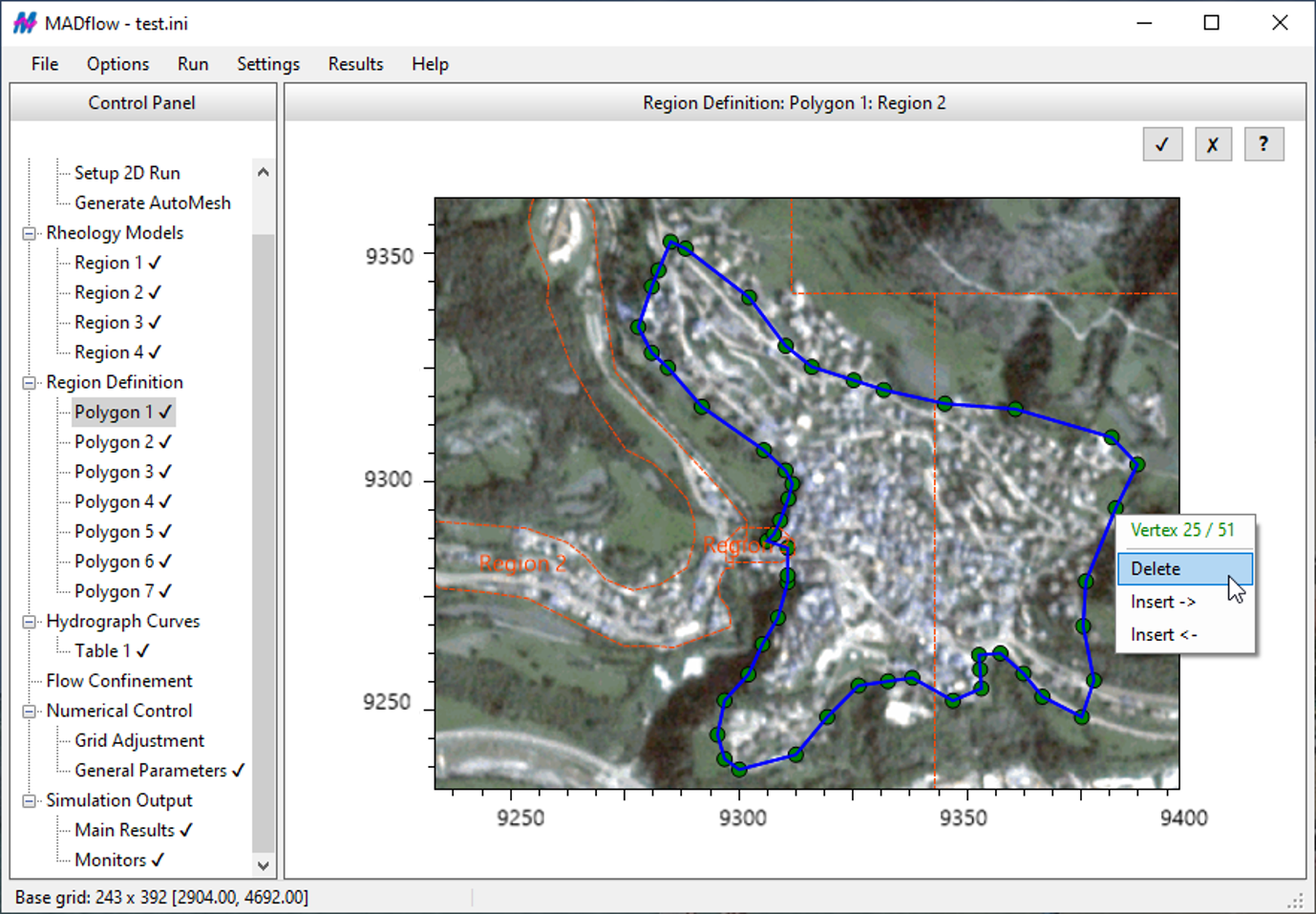
Each data item or group within the textual control file is prefaced by a descriptive keyword indicating its purpose (see example below). MADflow adopts a multi-region approach, enabling the application of different rheologies with specific parameters across zones defined by arbitrary complex polygons in plain text syntax. Boundary conditions such as out-flow or no-flow can be assigned at the domain (or no-data) boundaries, and simulations can be halted and resumed at any point during execution.
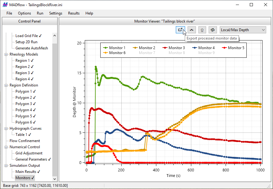
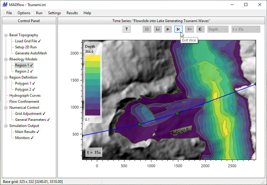
The software supports two flow mobilization methods — Source-zone and Discharge-tables — which can be used simultaneously within a single run. The Source-zone method outputs cumulative released volume and outflow rate from the source zone (i.e., hydrograph) as part of the simulation results. Both methods allow for spatial and temporal variation of volumetric solid concentration (Cv), if applicable. Key outputs typically include the area influenced by runout, velocity/flux time histories (at user-specified intervals) during runout, and distributions of flow depth during runout and deposition. Additionally, results can be extracted for specific points or line segments of interest (monitor points or lines).
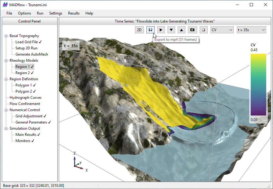
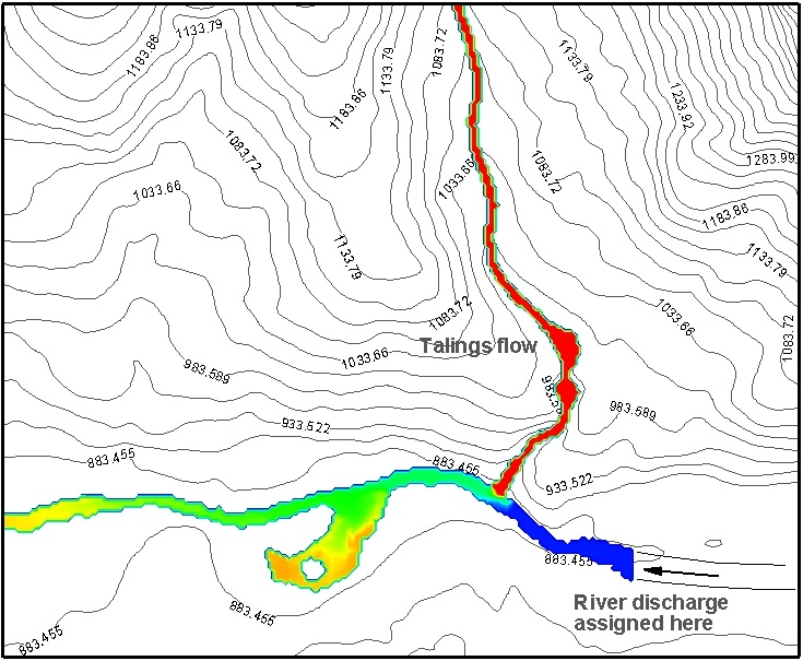
In the case of the Discharge-table method, influx sections can be positioned anywhere within the computational domain, independent of grid alignment. There are no constraints on the number of discharge tables that can be applied, and MADflow accurately tracks released volumes at specified times. Depending on the chosen rheological model, spatially varying Cv influences and adjusts flow properties accordingly. An illustrative example (shown above) demonstrates Cv mixing in a scenario involving tailings flow (Cv = 0.45, marked in red) and river flow (Cv = 0.0, marked in blue).
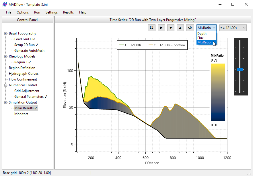
MADflow features an intuitive graphical user interface (GUI) on Windows, enabling convenient model building and efficient simulation analysis.